LMI Exposure Time Calculator
Status: Completed 2025-07-22
Overview
The Basics of the Exposure Time Calculator
The LDT/LMI Exposure Time Calculator (ETC) is based upon the Appendix in the Direct Imaging Manual for Kitt Peak (Massey et al. 1992, 2002) [1]. The signal-to-noise ratio (SNR) is calculated as follows. First, the signal is simply the count rate (\(e^-\)/sec) from the star \(N_*\) measured through some aperture times the exposure time \(t\). The noise is make up of three components, which are added in quadrature:
The photon noise from the star itself, \(\sqrt{N_*\times t}\).
The photon noise from the sky, \(\sqrt{S\times p \times t}\), where S is the count rate per pixel (\(e^-\)/sec/pixel) and \(p\) is the number of pixels in the measuring aperture.
The read-noise from the device \(\sqrt{p}\times R\) in the measuring aperture, where \(R\) is the read-noise per pixel.
Put this all together and we have:
In doing this, we have ignored dark current (which is usually negligible), and flat-fielding errors.
Where do the individual parameters come from?
We assume that the number of pixels \(p\) is dependent on the seeing, and that the astronomer will always measure the brightness of a star using a near-optimal measuring aperture, i.e., one that has a radius that is about \(0.67\times\) the full-width at half-maximum (fwhm) [2]. In that case the number of pixels \(p\) will be \(\pi \times (0.67 \times {\rm fwhm})^2 = 1.4 \times {\rm fwhm}^2\). If the number of pixels is less than 9, we impose a minimal value of 9, corresponding to a radius of 2.5 pixels.
With each of the telescope/CCD combinations, we have measured the observed count rates (\(e^-\)/sec) and then normalized the values to a \(U=B=V=R=I=20\) mag star observed, correcting for extinction to outside the earth’s atmosphere (airmass \(X=0.0\)). Let’s call these values \(N_{\rm 20}\). Thus if we want to know \(N_*\) for a star of magnitude m that we plan to observe at an airmass of \(X\) we compute:
The sky value \(S\) (in \(e^-\)/sec/pixel) is a little tricker to compute.
First, it clearly is a function of lunar phase, particularly at the
bluer wavelengths. Massey et al. (1992, 2002) have tabulated the sky
brightness (in mag/arcsec\(^2\)) at various lunar phases, and
Frank Valdes performed a simple low order fit to these for use in
ccdtime, and we adopt these values here. Yes, the actual sky brightness
depends (a lot) on how far away from the moon you are pointing, but we
are trying to give reasonable ballpark estimates here. So, we know the
sky brightness \(s\) in mag/arcsec\(^2\). The counts you
expect from the sky per arcsec\(^2\) is thus
\(N_{\rm 20} \times 10^{-(s-20)/2.5}\). The area of a pixel is the
scale\(^2 \times\) binining\(^2\) (where the scale is in
arcsec/pixel) and so
The read-noise \(R\) is a value you measure in the lab (and at the telescope), and is typically \(\sim\)4-7 \(e^-\).
How do we do it?
Given any two parameters, we want the third. Here are the equations we use, given the above.
Case 1: Given a magnitude and a SNR, what exposure time do we want?
This is dealt with explicitly in Massey et al. (1992, 2002). If we solve Equation (1) for \(t\), we find ourselves with our old friend the quadratic equation:
where
Case 2: Given a magnitude and exposure time, what SNR to we achieve?
This is the easiest case: we just plug our values into Equation (1).
Case 3: Given a SNR and exposure time, what magnitude do we reach?
This requires first solving Equation (1) for \(N_*\), which again requires the quadratic equation:
where
Once we have \(N_*\) we must turn it into a magnitude:
That’s the brightness of a star outside the earth’s atmosphere. But we aren’t going to go as faint as that, as we are observing at some finite airmass \(X\). So,
Output
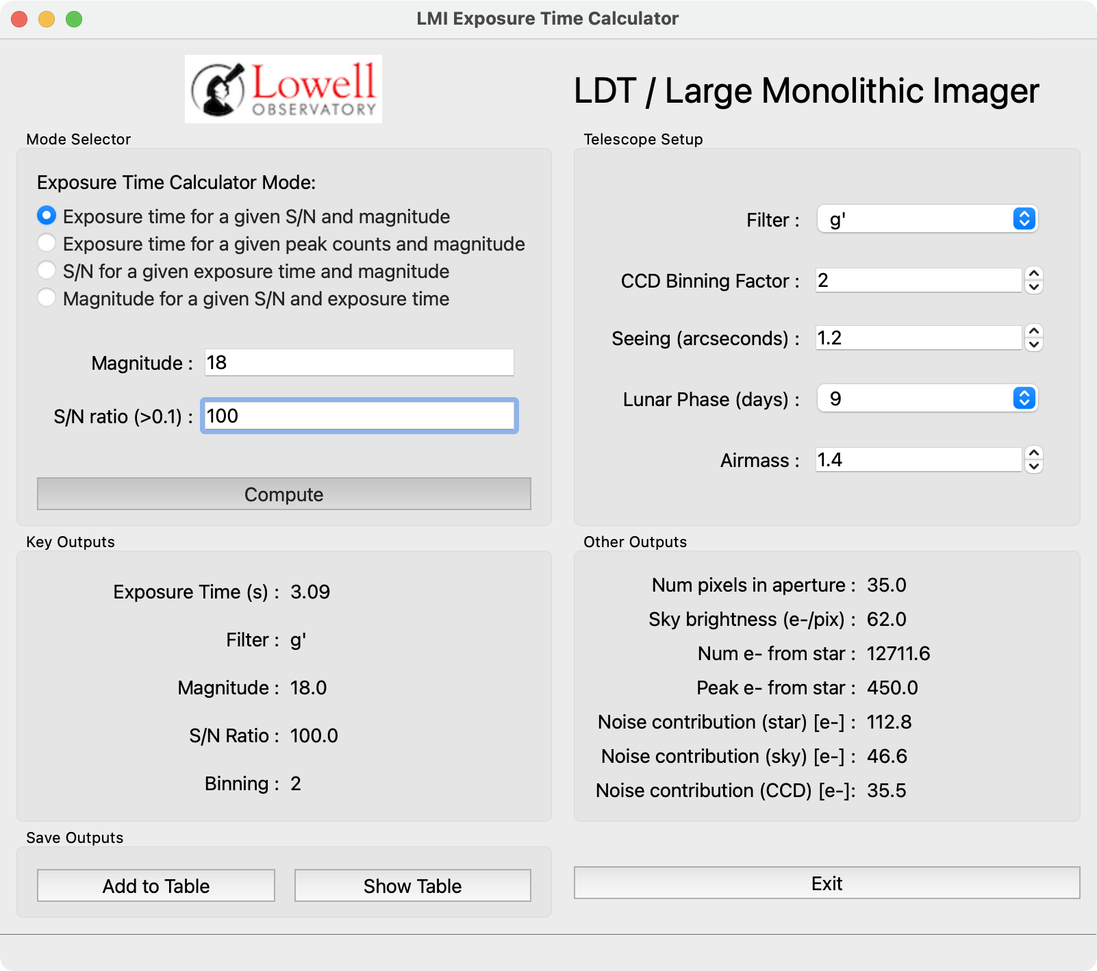
We give the bandpass, magnitude, S/N, and exposure time, irrespective of which two were input and which one is output. We also include the number of pixels in the measuring aperture, the sky brightness (in \(e^-\)/pixel), the number of e from the star, the peak number of \(e^-\) from the star (see below), and the noise contributions from the three components.
The peak number of counts from the star \(P\) will be (roughly):
where the fwhm is in pixels.
Table 1. Count Rates Assumed \(N_{20}\) \(e^-\) /sec/image |
|||||||
|---|---|---|---|---|---|---|---|
Tel/Inst |
U |
B |
V |
R |
I |
VR |
Readnoise |
LDT/LMI |
100 |
730 |
680 |
670 |
450 |
990 |
7.0 |
Hall/NASA42 |
3.1 |
17.1 |
17.5 |
19.7 |
12.8 |
25.0 |
4.6 |
The above text was written by Phil Massey. The original code for the LMI exposure time calculator was written and tested by Kathryn Neugent.
Usage
The script usage can be displayed by calling the script with the
-h option:
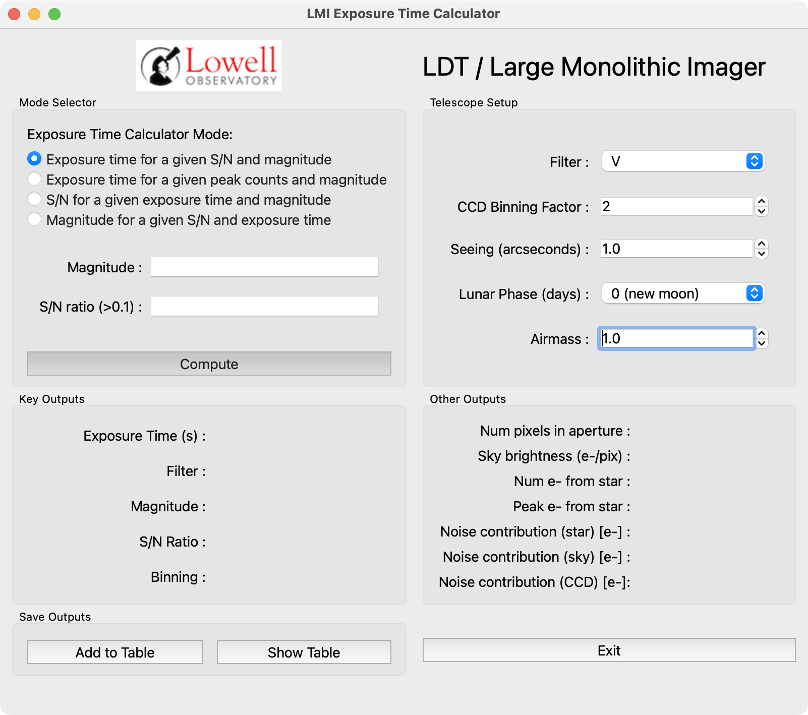
When launched, the GUI presents a window as in Fig. 1.

Fig. 1 – The lmi_etc GUI at startup.
Observation options may be set in the box at the top right (filter, seeing, etc.). Basic default values are loaded at startup. The filter set is the one for which basic values (star counts per second at \(m_v=20\), extinction, etc.) have been measured.
Select one of the four modes in the top-left box for the computation. The input boxes below the radio buttons will display the proper input fields for the chosed mode. Clicking “Compute” will call the proper calculation routine based on the mode and will display all of the computed values in the two “Output” boxes (see Fig. 2).

Fig. 2 – The lmi_etc GUI displaying computed values.
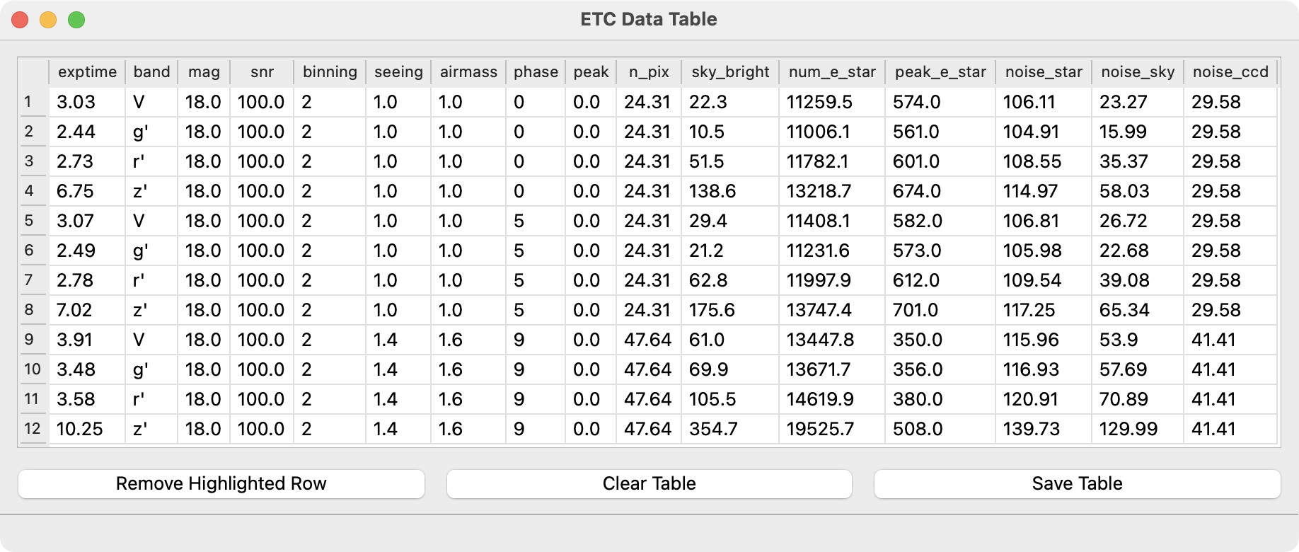
Because many observers use exposure time calculators to help plan an observing run, this tool has the added feature of saving the calculated values for each setup to disk. After performing a calculation, the user may add the presently displayed values to a table using the “Add to Table” button. The table (see Fig. 3) may be shown / hidden using the “Show Table” button.

Fig. 3 – The lmi_etc data table after adding several proposed observations.
Within the data table window, the user may remove lines (e.g., accidentally duplicated entries), clear the entire table and start over, or save the displayed table to disk.
At present, the save options are:
AstroPy’s Enhanced Character-Separated Values format (
.ecsv)standard comma-separated values format (
.csv)AstroPy’s fixed-width text table (
.txt)FITS binary table (
.fits)